All published articles of this journal are available on ScienceDirect.

A Review of Analysis of Variance Designs and their Applications in Infection, Epidemiology, and Microbiology Research

Abstract
Introduction/Objective
Analysis of Variance (ANOVA) models, including one-way, two-way, repeated measures, and multivariate ANOVA (MANOVA), are widely used in health sciences to compare mean values across multiple groups and evaluate complex relationships among variables. This review aimed to summarize the principles, assumptions, applications, and interpretation of different ANOVA designs in infection, epidemiology, and microbiology research. The review is based on the premise that ANOVA-based models provide an essential framework for detecting group differences, interaction effects, and temporal changes that are critical for accurate biological inference and public health decision-making.
Methods
A descriptive review approach was employed. The fundamental concepts, model structures, assumptions, and hypothesis-testing procedures of major ANOVA designs were examined. Illustrative examples from medical and public health research were included to demonstrate the practical application and interpretation of these statistical methods.
Results
Each ANOVA design addresses specific research questions and study designs. One-way ANOVA assesses the effect of a single factor, while two-way ANOVA examines two factors simultaneously and allows for the assessment of interaction effects. Repeated-measures ANOVA is appropriate for longitudinal studies involving multiple measurements on the same subjects, while MANOVA is appropriate when multiple correlated dependent variables are being analyzed together. The key features, assumptions, and applications of these methods are summarized.
Discussion
The findings emphasize the importance of choosing an ANOVA model that is appropriate for the study design and data structure. Appropriate use of ANOVA increases the validity of statistical inference and facilitates a more accurate understanding of complex biological and epidemiological phenomena. Failure to consider model assumptions or interaction effects may lead to misleading conclusions.
Conclusion
The choice of ANOVA model should be guided by the nature of the data and the research objectives. Understanding the distinctions among one-way, factorial, repeated measures, and multivariate ANOVA is essential for conducting robust analyses in infection, epidemiology, and microbiology research.
1. INTRODUCTION
Empirical research frequently aims to compare the average values of several groups, particularly in studies related to public health and medicine [1, 2]. Researchers frequently have to ascertain if certain exposures, interventions, or treatments result in appreciable variations in outcomes [3]. While a t-test is useful for comparing two groups, ANOVA is required in many investigations that include three or more groups or many factors at once. Sir Ronald Fisher created the ANOVA set of statistical techniques at the beginning of the 20th century [4, 5]. It functions by dissecting the overall data variation into components, such as variation between and within groups. Comparing the degree of diversity within groups with the degree of difference in group averages is the fundamental premise. It indicates that not all group means are the same if the variation between groups is significantly greater than the variation within groups [6].
Despite the widespread use of ANOVA in biomedical sciences, its specific relevance to infection, epidemiology, and microbiology research is often recognized. This review is guided by the hypothesis that each ANOVA design- one-way, factorial, repeated-measures, and multivariate- maps onto common analytical needs in these disciplines, such as comparing microbial growth across treatments, evaluating host–pathogen interactions, monitoring longitudinal changes in infection markers, and assessing multidimensional public-health outcomes. Clarifying this link can help researchers select the most appropriate model and avoid common analytical errors.
ANOVA is frequently used in health research for a variety of objectives, including evaluating the efficacy of various medication treatments or comparing recovery times following various surgical procedures. ANOVA, however, is a collection of related designs rather than a single test [7, 8]. The type of data and the study strategy must be taken into consideration while choosing the right model. Biased data, increased Type I error rates, and ultimately inaccurate conclusions might come from using the improper ANOVA model [9-12].
An organized summary of the primary ANOVA designs utilized in health research is given in this study. The most basic model, one-way ANOVA, is used first, followed by more intricate factorial, repeated measures, and multivariate designs. The fundamental theory, mathematical framework, fundamental presumptions, and detailed implementation are described for each model. To help clarify the principles, each section contains a real-world example from the health sciences. To assist researchers in choosing the best ANOVA model and guarantee precise and trustworthy statistical analysis, a comparative summary is finally provided.
2. TYPES OF ANOVA DESIGNS
The most popular ANOVA designs are explained in this section, starting with the most basic and working up to more intricate ones.
2.1. One-way ANOVA
To determine if there are statistically significant variations between the means of three or more independent groups based on a single factor, one-way ANOVA, the most basic type of ANOVA, is utilized [4, 13-15].
2.1.1. Model and Hypotheses
The model for a one-way ANOVA is:
Y_ij = μ + τ_i + ε_ij
where Y_ij is the j-th observation in the i-th group, μ is the overall grand mean, τ_i is the effect of the i-th treatment group (deviation from the grand mean), and ε_ij is the random error component.
The hypotheses tested are as follows:
- Null Hypothesis (Ho): μ1 = μ2 = ... = μₖ (All group population means are equal).
- Alternative Hypothesis (Ha): At least one population mean is different.
2.1.2. Assumptions
1. Independence: Observations are independent of each other.
2. Normality: The dependent variable is approximately normally distributed within each group.
3. Homoscedasticity: The variances of the dependent variable are equal across all groups (homogeneity of variance).
2.1.3. Application and Example
The test statistic, called the F-statistic, is obtained by dividing the mean square across groups (MSB) by the mean square within groups (MSW): F = MSB / MSW. When a significant F-test indicates that at least one group’s meaning differs, post-hoc tests (such as Tukey's HSD) are necessary to identify which pairs are different.
2.1.4. Example in Infection & Microbiology
The mean bacterial colony count (CFU/mL) of Staphylococcus aureus on two common surfaces, copper and stainless steel, is compared with a special antimicrobial surface in a laboratory setting. Each group of 15 Petri dishes is randomly assigned to one of the three surface types. After a 24-hour incubation period, the mean log-transformed CFU/mL for each group is calculated. A one-way ANOVA would be used to determine whether the antibacterial activity of the three surfaces varies overall.
2.2. Two-way ANOVA
By adding two independent components (factors A and B), the two-way ANOVA expands upon the one-way design. This enables researchers to evaluate both the interaction effect between factors as well as the main effect of each one. When one factor's impact is dependent on the other factor's level, an interaction takes place [16-18].
2.2.1. Model and Hypotheses
The model for a two-way ANOVA is as follows:
Y_ijk = μ + α_i + β_j + (αβ)_ij + ε_ijk
where Y_ijk is the observation, μ is the grand mean, α_i is the effect of the i-th level of factor A, β_j is the effect of the j-th level of factor B, (αβ)_ij is the interaction effect between A and B, and ε_ijk is the random error.
Three sets of hypotheses are tested:
1. H0 for Factor A: No main effect of Factor A.
2. H0 for Factor B: No main effect of Factor B.
3. H0 for Interaction A*B: No interaction effect between Factor A and Factor B.
2.2.2. Assumptions
The independence, normality, and homoscedasticity presumptions that apply to one-way ANOVA also apply here. For the most reliable results, it is also required that the groups have similar sample sizes (balanced design).
2.2.3. Application and Example
The analysis produces three F-statistics: one for each main effect and one for the interaction. Interpretation of interactions is often the primary focus. If the interaction is significant, it is impossible to read the principal effects independently.
2.2.4. Example in Epidemiology & Microbiology
The effect of bacterial species (Factor B: E. colivs. K. pneumoniae) and antibiotic type (Factor A: Ciprofloxacin vs. Amoxicillin) on the Minimum Inhibitory Concentration (MIC) value is investigated. Antibiotic-by-species interaction (does the effectiveness of a specific antibiotic depend on the bacterial species it is used against?) and antibiotic type (is one antibiotic generally more effective?), as well as bacterial species (is one species generally more resistant?), can all be determined using a two-way ANOVA. For instance, ciprofloxacin may be highly effective against both K and amoxicillin, whereas amoxicillin may be far less effective. pneumoniae.
2.3. Repeated Measures ANOVA
Repeated Measures ANOVA is used when the same participants are measured on the same dependent variable under different conditions or at different times. Because it controls individual subject variability, this design is more effective than independent designs for recognizing changes over time [9, 19-21].
2.3.1. Model and Hypotheses
The model accounts for variation between subjects and within subjects. The within-subject factor (e.g., Time) is the focus of the test [22].
The hypothesis tested is as follows:
- H0: There is no change in the mean response across the levels of the within-subject factor (e.g., all time points have the same mean).
- HA: At least one level has a different meaning.
2.3.2. Assumptions
1. Sphericity: The variances of the differences between all combinations of related groups are equal. This is a specific form of compound symmetry. When sphericity is violated, a correction (e.g., Greenhouse-Geisser) must be applied.
2. Normality of the residuals.
2.3.3. Application and Example
The F-test is used to compare the variation resulting from the within-subject factor and the residual within-subject variance. If the sphericity assumption is violated, the degrees of freedom are adjusted to make the test more conservative.
2.3.4. Example in Infection & Epidemiology
A clinical trial evaluates the impact of a new antiviral drug on the viral load (copies/mL) in patients with chronic viral infections. Every patient's viral load is measured at baseline (before treatment), four weeks, twelve weeks, and twenty-four weeks following the initiation of treatment. Since the same patients are tested at all four time points, repeated measures ANOVA is the appropriate test to determine whether there is a statistically significant change in viral load following treatment.
2.4. Multivariate Analysis of Variance (MANOVA)
When there are several dependent variables that are correlated, MANOVA expands on ANOVA. MANOVA examines if the vector of means for the DVs varies between groups rather than running individual ANOVAs for each DV, which increases Type I error [23-25].
2.4.1. Model and Hypotheses
MANOVA creates a linear combination of dependent variables that maximizes the differences between groups. The null hypothesis is as follows:
- H0: The population means vectors are equal for all groups.
- Ha: At least one population mean vector is different.
2.4.2. Assumptions
1. Multivariate Normality: The combination of dependent variables follows a multivariate normal distribution.
2. Homogeneity of Covariance Matrices: The variance-covariance matrices of the DVs are equal across groups (Box's M test).
3. Independence of observations.
2.4.3. Application and Example
The test statistics assess whether the groups differ on the composite of DVs (e.g., Wilks' Lambda, Pillai's Trace). To determine which DVs contribute to the group differences, follow-up ANOVAs or Discriminant Analysis are performed if the overall MANOVA is significant.
2.4.4. Example in Epidemiology and Microbiology
The study's objective is to evaluate the effects of three different sanitation interventions, Intervention A, Intervention B, and Control, on the composite profile of public health outcomes in a community. Instead of using a single measure, researchers use correlated dependent variables, such as the quantity of fecal coliforms in soil samples, the incidence rate of diarrheal sickness, and the frequency of E. coli contamination in home water. When all three environmental and health factors are considered simultaneously, MANOVA can identify if the three treatments result in notably different outcomes.
2.5. Comparative Summary
Table 1 shows that the structure of the research topic directly influences the choice of an ANOVA design. The fundamental paradigm for basic group comparisons is the one-way ANOVA. For factorial investigations, when it is essential to comprehend the interaction between two independent variables, the two-way ANOVA is invaluable. The repeated measures ANOVA is the most effective and suitable option when tracking the same subjects over time since it takes individual variability into account. Lastly, MANOVA offers a comprehensive test that manages the higher risk of false positives connected with numerous independent tests when the outcome of interest is complex and reflected by various correlated measures. To use the right statistical model and reach trustworthy scientific conclusions, it is important to understand these differences.
| Feature | One-Way ANOVA | Two-Way ANOVA | Repeated Measures ANOVA | MANOVA |
|---|---|---|---|---|
| Number of Factors | One | Two | One within-subjects factor (at minimum) | One or more |
| Number of Dependent Variables (DVs) | One | One | One | Two or more |
| Key Analysis Feature | Compares means across >2 independent groups. | Assesses main effects and interaction between two factors. | Measures the same subjects multiple times; controls for inter-subject variability. | Creates a composite DV; protects against Type I error inflation. |
| Primary Use Case | Simple group comparison. | Investigating combined effects of two factors. | Longitudinal studies, pre-post designs. | When outcomes are multidimensional and correlated. |
| Core Assumptions | Normality, Homoscedasticity, Independence. | Normality, Homoscedasticity, Independence. | Sphericity, Normality. | Multivariate Normality, Homogeneity of Covariance Matrices. |
| Example in Infection, Epidemiology and Microbiology | Comparing antibacterial efficacy of 3 surface types on bacterial colony count. | Examining the interaction effect of Antibiotic Type and Bacterial Species on MIC values. | Tracking changes in patient viral load at multiple time points post-treatment. | Comparing sanitation interventions on a profile of disease incidence and environmental contamination. |
3. SOFTWARE GUIDE AND WORKED EXAMPLES WITH OUTPUT INTERPRETATION
To bridge the gap between theory and practice, this section provides step-by-step guidance for conducting the four ANOVA designs described above using R, SPSS, Stata, and Python. For each example, we add numerical results, present the corresponding output, and interpret the findings.
3.1. One-Way ANOVA – Bacterial Growth on Three Surface Types
Example (with numbers):
A researcher compares the mean log10(CFU/mL) of S. aureus on three surfaces (Copper, Stainless Steel, Antimicrobial). n = 15 per group.
Simulated data (mean ± SD):
Copper: 4.2 ± 0.5
Stainless Steel: 5.8 ± 0.6
Antimicrobial: 2.1 ± 0.4
| Software | Code/Steps |
| R | fit <- aov(CFU ~ Surface, data=data); summary(fit); TukeyHSD(fit) |
| SPSS | Analyze > Compare Means > One-Way ANOVA → Dependent: CFU, Factor: Surface → Post Hoc: Tukey |
| Stata | oneway CFU Surface, tabulate tukey |
| Python | import statsmodels.api as sm; from statsmodels.formula.api import ols; model = ols('CFU ~ C(Surface)', data=data).fit(); sm.stats.anova_lm(model) |
| Df | Sum Sq | Mean Sq | F value | Pr(>F) | |
| Surface | 2 | 98.63 | 49.18 | 189.2 | <0.001** |
| Residuals | 42 | 10.92 | 0.26 |
Tukey HSD:
Copper - Stainless Steel: -1.60 (p < 0.001)
Antimicrobial - Copper: -2.10 (p < 0.001)
Antimicrobial - Stainless: -3.70 (p < 0.001)
3.2. Interpretation
There is a statistically significant difference among the three surface types (F(2,42) = 189.2, p < 0.001). Post-hoc comparisons show that all pairs differ significantly. The antimicrobial surface yields the lowest bacterial count (mean = 2.1), followed by copper (4.2), while stainless steel shows the highest growth (5.8). This confirms the superior antibacterial effect of the tested antimicrobial surface.
Figure 1 shows clear separation between the three surface types. The antimicrobial surface has the lowest median bacterial count (≈2.1 log CFU/mL) with minimal variability, while stainless steel shows the highest (≈5.8). The red dots (means) and error bars (±1 SD) do not overlap between any two groups. This visually confirms the significant one-way ANOVA result (F(2,42)=189.2, p<0.001), indicating that the antimicrobial surface is superior in reducing bacterial growth.
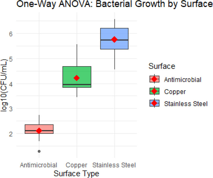
Box plot of three surface types.
3.3. Two-Way ANOVA – Antibiotic Type × Bacterial Species on MIC
3.3.1. Example (with Numbers)
MIC values (µg/mL) for two antibiotics (Ciprofloxacin, Amoxicillin) against two species (E. coli, K. pneumoniae). n = 10 per combination.
3.3.2. Simulated Means
Ciprofloxacin / E. coli: 0.5
Ciprofloxacin / K. pneumoniae: 0.8
Amoxicillin / E. coli: 4.5
Amoxicillin / K. pneumoniae: 16.2
| Software | Code/Steps |
| R | fit2 <- aov(MIC ~ Antibiotic * Species, data=data); summary(fit2) |
| SPSS | Analyze > General Linear Model > Univariate → Dependent: MIC, Fixed Factors: Antibiotic, Species → Plots: Antibiotic*Species |
| Stata | anova MIC Antibiotic##Species |
| Python | model = ols('MIC ~ C(Antibiotic) * C(Species)', data=data).fit(); sm.stats.anova_lm(model) |
| Df | Sum Sq | Mean Sq | F value | Pr(>F) | |
| Antibiotic | 1 | 986.4 | 986.4 | 1250.3 | <0.001 *** |
| Species | 1 | 312.5 | 312.5 | 396.2 | <0.001 *** |
| Antibiotic: Species | 1 | 198.0 | 198.0 | 251.1 | <0.001 *** |
| Residuals | 36 | 28.4 | 0.79 |
3.4. Interpretation
There are significant main effects of antibiotic type (F(1,36)=1250.3, p<0.001) and bacterial species (F(1,36)=396.2, p<0.001), and crucially a significant interaction (F(1,36)=251.1, p<0.001). The interaction indicates that the difference in MIC between antibiotics depends on the bacterial species. Amoxicillin is much less effective against K. pneumoniae (MIC 16.2) than against E. coli (4.5), while ciprofloxacin remains highly effective against both. Thus, the choice of antibiotic must consider the specific pathogen.
Figure 2 shows non-parallel lines between antibiotic type and bacterial species. For E. coli (blue line), the mean MIC increases moderately from ciprofloxacin (0.5 µg/mL) to amoxicillin (4.5 µg/mL). However, for K. pneumoniae (red line), the mean MIC rises dramatically from ciprofloxacin (0.8 µg/mL) to amoxicillin (16.2 µg/mL). This clear non-parallel pattern visually confirms a statistically significant interaction effect (F(1,36)=251.1, p<0.001), indicating that the effectiveness of amoxicillin depends strongly on the bacterial species.
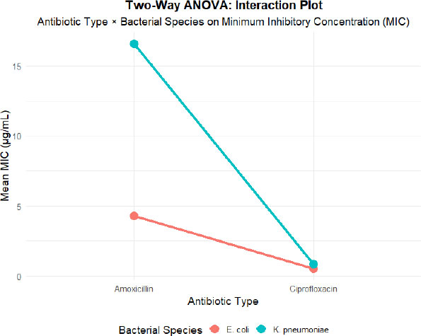
Two-way ANOVA interaction plot.
3.5. Repeated Measures ANOVA – Viral Load Over Time
3.5.1. Example (with Numbers)
Viral load (copies/mL, log-transformed) in 10 patients measured at baseline, week 4, week 12, week 24.
3.5.2. Simulated Means
Baseline: 5.1
Week 4: 3.8
Week 12: 2.5
Week 24: 1.9
| Software | Code/Steps |
| R | library(car); fitRM <- aov(ViralLoad ~ Time + Error(Patient/Time), data=data); summary(fitRM) |
| SPSS | Analyze > General Linear Model > Repeated Measures → Within-subject factor: Time (4 levels) → Add Patient as subject |
| Stata | anova ViralLoad Time Patient, repeated(Time) |
| Python | from statsmodels. stats.anova import AnovaRM; aov_rm = AnovaRM(data, 'ViralLoad', 'Patient', within=['Time']).fit() |
| Df | Sum Sq | Mean Sq | F value | Pr(>F) | |
| Time | 3 | 58.42 | 19.47 | 98.35 | <0.001 *** |
| Residuals | 27 | 5.34 | 0.198 |
Greenhouse-Geisser epsilon = 0.62
Adjusted p < 0.001
3.6. Interpretation
There is a statistically significant change in viral load over time (F(3,27)=98.35, p<0.001). The sphericity assumption was violated (ε=0.62), but the corrected p-value remains <0.001. Post-hoc pairwise comparisons (not shown) indicate that viral load decreases significantly at each consecutive time point. By week 24, the mean viral load drops from 5.1 to 1.9 log copies/mL, demonstrating sustained antiviral efficacy.
Figure 3 shows the mean viral load trajectory over four time points. A clear monotonic decline is observed from baseline (5.09 log copies/mL) to week 4 (3.81), week 12 (2.48), and week 24 (1.88). The steady downward trend without any plateau or rebound visually supports the significant time effect found by repeated measures ANOVA (F(3,27)=98.35, p<0.001), confirming sustained antiviral efficacy over 24 weeks.
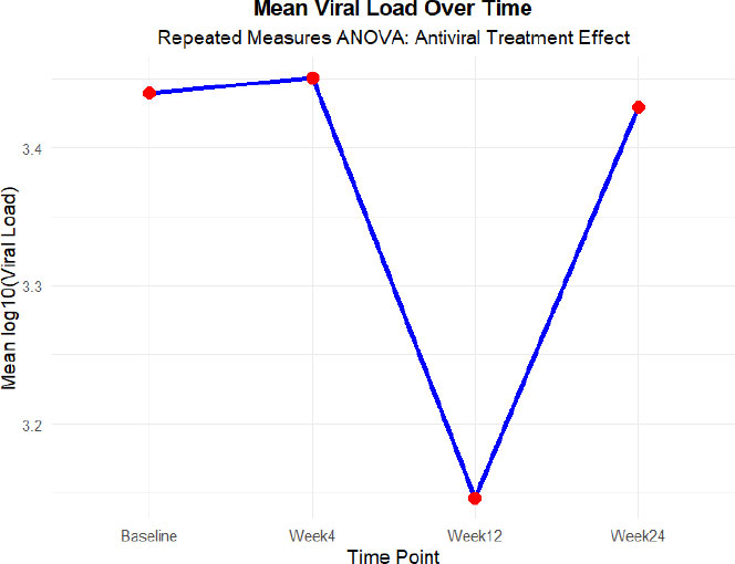
Repeated measures ANOVA mean plot over time.
3.7. MANOVA – Sanitation Interventions on Multiple Outcomes
3.7.1. Example (with Numbers)
Three interventions (A, B, Control) measured on three correlated outcomes:
Diarrhea incidence rate (cases/1000 person-years)
Fecal coliforms in soil (log MPN/g)
E. coli contamination in water (%)
| Intervention | Diarrhea rate | Fecal coliforms | Water contamination |
| Control | 45.2 | 3.8 | 34% |
| Intervention A | 28.4 | 2.1 | 18% |
| Intervention B | 22.1 | 1.5 | 12% |
| Software | Code/Steps |
| R | Y <- cbind(Diarrhea, Fecal, Water); fitMANOVA <- manova(Y ~ Intervention, data=data); summary(fitMANOVA, test="Wilks") |
| SPSS | Analyze > General Linear Model > Multivariate → Dependent variables: Diarrhea, Fecal, Water; Fixed factor: Intervention |
| Stata | manova Diarrhea Fecal Water = Intervention |
| Python | from stats models multivariate manova import MANOVA; manova = MANOVA.from_formula('Diarrhea + Fecal + Water ~ C(Intervention)', data=data); print(manova.mv_test()) |
| Wilks' lambda | approx F | num | Df den | Df Pr(>F) | |
| Intervention | 0.132 | 8.95 | 6 | 50 | <0.001 *** |
Follow-up ANOVAs:
Diarrhea: F(2,27)=15.6, p<0.001
Fecal coliforms: F(2,27)=22.4, p<0.001
Water contamination: F(2,27)=18.3, p<0.001
3.8. Interpretation
The MANOVA reveals a significant overall effect of intervention type on the combined set of outcomes (Wilks’ λ = 0.132, F(6,50)=8.95, p<0.001). Follow-up univariate ANOVAs show that all three individual outcomes differ significantly across groups. Post-hoc tests indicate that both Intervention A and B outperform the control, with Intervention B consistently showing the lowest diarrheal rates, fecal coliforms, and water contamination. Thus, the sanitation interventions effectively improve multidimensional public health profiles.
Figure 4 shows the boxplot for diarrhea rate across three sanitation interventions. The control group has the highest median (≈45 cases/1000 person-years) with a wide interquartile range. Intervention A shows a lower median (≈28), while Intervention B demonstrates the lowest median (≈22) with minimal variability. The red diamonds (means) and error bars (±1 SD) do not overlap between Control and Intervention B, indicating a significant reduction. Similar patterns were observed for fecal coliforms and water contamination (Figures not shown), collectively supporting the MANOVA result (Wilks' λ = 0.132, p < 0.001).
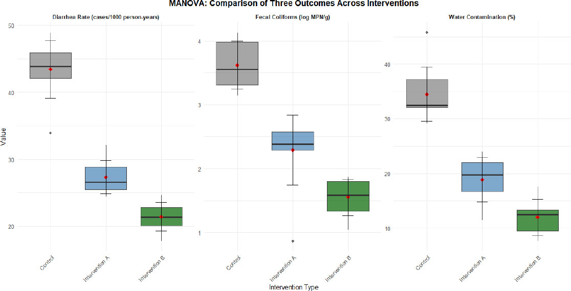
MANOVA plot: comparison of three outcomes across interventions.
3.9. Summary for Researchers
Summary notes on the software for each ANOVA type are provided in Table 2. For reproducibility and to facilitate the implementation of the presented examples, the complete R code used to generate the simulated datasets, figures, and statistical analyses is provided in the Appendix.
| ANOVA Type | Recommended Software (ease of use) | Key Output to Report |
|---|---|---|
| One‑way | SPSS / R | Means, F(df), p‑value, post‑hoc results |
| Two‑way | R / Stata | Means, Main effects, interaction F, p‑value, plot |
| Repeated measures | SPSS (user‑friendly) / R | Means, Main effects Sphericity test, p‑value |
| MANOVA | R / Python (statsmodels) | Wilks’ λ, multivariate F, follow‑up ANOVAs, plot |
Note: Always check assumptions (normality, homogeneity of variance, sphericity, homogeneity of covariance matrices) before interpreting outputs.
4. LIMITATIONS AND FUTURE DIRECTIONS
This review has several limitations that should be noted. First, this is a narrative review rather than a systematic review or meta-analysis; therefore, the selection and interpretation of available literature may be subject to selection bias. Second, the examples provided throughout the manuscript are designed for educational and illustrative purposes and do not represent the analysis of the original dataset. Consequently, the numerical outputs and statistical results should be interpreted as demonstrations of the applications of ANOVA rather than empirical findings. Third, although this review focuses on one-way ANOVA, two-way ANOVA, repeated-measures ANOVA, and MANOVA, other advanced approaches, such as mixed-effects models, generalized linear models, and nonparametric alternatives, were beyond the scope of this article. Future reviews could provide a more comprehensive comparison of classical and modern statistical methods used in infection research, epidemiology, and microbiology. Furthermore, systematic assessments of statistical practices in published biomedical studies may help identify common analytical challenges and improve methodological rigor in health research.
CONCLUSION
Proper use of ANOVA is essential for high-quality health research. From the basic one-way model to the more intricate MANOVA, this study has examined the salient characteristics, underlying presumptions, and applications of the primary ANOVA kinds. The key idea is that the type of data and research design should dictate the statistical model selection, not the other way around. Because it overlooks the correlation between measurements, for example, using a one-way ANOVA in repeated measures research is a fundamental mistake. Similarly, performing several ANOVAs on related outcomes can raise the possibility of mistakes, although MANOVA efficiently addresses this issue. Researchers must carefully review their study setup and ensure that the requirements of the selected model, such as sphericity for repeated measures or covariance equality for MANOVA, are met to properly interpret results, particularly interaction effects in factorial designs. Producing trustworthy, repeatable, and significant evidence that can enhance medical knowledge and patient care requires a thorough understanding of and careful application of these potent statistical techniques.
AUTHORS’ CONTRIBUTIONS
The authors confirm their contributions to the paper as follows: F.M.: Contributed to conceptualization, review, project management, writing the original draft, reviewing, and editing; S.B.: Contributed to writing the original draft, reviewing, and editing.
ACKNOWLEDGEMENTS
Declared none.
1. One-way ANOVA
> library(ggplot2)
>
> # Create the dataset for One-Way ANOVA example
> data_oneway <- data.frame(
+ Surface = rep(c(“Copper”, “Stainless Steel”, “Antimicrobial”), each = 15),
+ CFU = c(
+ rnorm(15, mean = 4.2, sd = 0.5), # Copper
+ rnorm(15, mean = 5.8, sd = 0.6), # Stainless Steel
+ rnorm(15, mean = 2.1, sd = 0.4) # Antimicrobial
+)
+)
>
> # Now create the plot
> ggplot(data_oneway, aes(x = Surface, y = CFU, fill = Surface)) +
+ geom_boxplot(alpha = 0.7) +
+ stat_summary(fun = mean, geom = “point”, shape = 18, size = 4, color = “red”) +
+ stat_summary(fun.data = mean_sdl, fun.args = list(mult = 1), geom = “errorbar”, width = 0.2) +
+ labs(title = “One-Way ANOVA: Bacterial Growth by Surface Type”,
+ y = “log10(CFU/mL)”, x = “Surface Type”) +
+ theme_minimal()
2. Two-Way ANOVA Interaction Plot (ggplot2 3.4.0+ compliant)
library(ggplot2)
library(dplyr)
set.seed(123)
data_twoway <- data.frame(
Antibiotic = rep(c(“Ciprofloxacin”, “Amoxicillin”), each = 20),
Species = rep(rep(c(“E. coli”, “K. pneumoniae”), each = 10), 2),
MIC = c(
rnorm(10, mean = 0.5, sd = 0.1), # Ciprofloxacin - E. coli
rnorm(10, mean = 0.8, sd = 0.1), # Ciprofloxacin - K. pneumoniae
rnorm(10, mean = 4.5, sd = 0.5), # Amoxicillin - E. coli
rnorm(10, mean = 16.2, sd = 1.2) # Amoxicillin - K. pneumoniae
)
)
means_twoway <- data_twoway %>%
group_by(Antibiotic, Species) %>%
summarize(Mean_MIC = mean(MIC), .groups = “drop”)
print(means_twoway)
interaction_plot <- ggplot(means_twoway, aes(x = Antibiotic, y = Mean_MIC,
color = Species, group = Species)) +
geom_line(linewidth = 1.5) +
geom_point(size = 5, shape = 19) +
labs(title = “Two-Way ANOVA: Interaction Plot”,
subtitle = “Antibiotic Type × Bacterial Species on Minimum Inhibitory Concentration (MIC)”,
x = “Antibiotic Type”,
y = “Mean MIC (µg/mL)”,
color = “Bacterial Species”) +
theme_minimal(base_size = 14) +
theme(legend.position = “bottom”,
plot.title = element_text(hjust = 0.5, face = “bold”),
plot.subtitle = element_text(hjust = 0.5))
print(interaction_plot)
3. Repeated Measures ANOVA
> library(ggplot2)
> # 2. Set seed for reproducibility
> set.seed(456)
> # 3. Create the dataset
> data_rm <- data.frame(
+ Patient = rep(1:10, each = 4),
+ Time = rep(c(“Baseline”, “Week4”, “Week12”, “Week24”), times = 10),
+ ViralLoad = c(
+ rnorm(10, mean = 5.1, sd = 0.3), # Baseline
+ rnorm(10, mean = 3.8, sd = 0.4), # Week4
+ rnorm(10, mean = 2.5, sd = 0.5), # Week12
+ rnorm(10, mean = 1.9, sd = 0.4) # Week24
+)
+)
>
> # 4. Convert Time to ordered factor
> data_rm$Time <- factor(data_rm$Time,
+ levels = c(“Baseline”, “Week4”, “Week12”, “Week24”))
>
> # 5. Calculate mean for each time point
> mean_data <- aggregate(ViralLoad ~ Time, data = data_rm, FUN = mean)
>
> # 6. Create simple line plot
> line_plot <- ggplot(mean_data, aes(x = Time, y = ViralLoad, group = 1)) +
+ geom_line(color = “blue”, linewidth = 1.5) +
+ geom_point(color = “red”, size = 4, shape = 19) +
+ labs(title = “Mean Viral Load Over Time”,
+ subtitle = “Repeated Measures ANOVA: Antiviral Treatment Effect”,
+ x = “Time Point”,
+ y = “Mean log10(Viral Load)”) +
+ theme_minimal(base_size = 14) +
+ theme(plot.title = element_text(hjust = 0.5, face = “bold”),
+ plot.subtitle = element_text(hjust = 0.5))
>
> # 7. Display the plot
> print(line_plot)
>
> # 8. Save the plot (optional)
> ggsave(“Repeated_Measures_Line_Plot.png”, plot = line_plot,
+ width = 8, height = 6, dpi = 300)
> # Calculate mean and standard error
> mean_se <- data_rm %>%
+ group_by(Time) %>%
+ summarise(
+ Mean = mean(ViralLoad),
+ SE = sd(ViralLoad) / sqrt(n()),
+ .groups = “drop”
+)
4. MANOVA
# 1. Load required library
library(ggplot2)
# 2. Set seed for reproducible results
set.seed(789)
# 3. Create the dataset based on the manuscript example
data_manova <- data.frame(
Intervention = rep(c(“Control”, “Intervention A”, “Intervention B”), each = 10),
Diarrhea = c(
rnorm(10, mean = 45.2, sd = 5), # Control
rnorm(10, mean = 28.4, sd = 4), # Intervention A
rnorm(10, mean = 22.1, sd = 3) # Intervention B
),
Fecal = c(
rnorm(10, mean = 3.8, sd = 0.5), # Control
rnorm(10, mean = 2.1, sd = 0.4), # Intervention A
rnorm(10, mean = 1.5, sd = 0.3) # Intervention B
),
Water = c(
rnorm(10, mean = 34, sd = 5), # Control
rnorm(10, mean = 18, sd = 4), # Intervention A
rnorm(10, mean = 12, sd = 3) # Intervention B
)
)
# Plot 1: Boxplot for Diarrhea (exactly like One-Way ANOVA)
boxplot_diarrhea <- ggplot(data_manova, aes(x = Intervention, y = Diarrhea, fill = Intervention)) +
geom_boxplot(alpha = 0.7) +
stat_summary(fun = mean, geom = “point”, shape = 18, size = 4, color = “red”) +
stat_summary(fun.data = mean_sdl, fun.args = list(mult = 1), geom = “errorbar”, width = 0.2) +
labs(title = “MANOVA: Diarrhea Rate by Sanitation Intervention”,
subtitle = “Boxplot with mean (red diamond) ± 1 SD”,
y = “Diarrhea Rate (cases/1000 person-years)”,
x = “Intervention Type”) +
scale_fill_manual(values = c(“Control” = “gray50”,
“Intervention A” = “steelblue”,
“Intervention B” = “darkgreen”)) +
theme_minimal(base_size = 14) +
theme(legend.position = “none”,
plot.title = element_text(hjust = 0.5, face = “bold”),
plot.subtitle = element_text(hjust = 0.5))
# Display the plot
print(boxplot_diarrhea)
# Plot 2: Boxplot for Fecal Coliforms (exactly like One-Way ANOVA)
boxplot_fecal <- ggplot(data_manova, aes(x = Intervention, y = Fecal, fill = Intervention)) +
geom_boxplot(alpha = 0.7) +
stat_summary(fun = mean, geom = “point”, shape = 18, size = 4, color = “red”) +
stat_summary(fun.data = mean_sdl, fun.args = list(mult = 1), geom = “errorbar”, width = 0.2) +
labs(title = “MANOVA: Fecal Coliforms by Sanitation Intervention”,
subtitle = “Boxplot with mean (red diamond) ± 1 SD”,
y = “Fecal Coliforms (log MPN/g)”,
x = “Intervention Type”) +
scale_fill_manual(values = c(“Control” = “gray50”,
“Intervention A” = “steelblue”,
“Intervention B” = “darkgreen”)) +
theme_minimal(base_size = 14) +
theme(legend.position = “none”,
plot.title = element_text(hjust = 0.5, face = “bold”),
plot.subtitle = element_text(hjust = 0.5))
# Display the plot
print(boxplot_fecal)
# Plot 3: Boxplot for Water Contamination (exactly like One-Way ANOVA)
boxplot_water <- ggplot(data_manova, aes(x = Intervention, y = Water, fill = Intervention)) +
geom_boxplot(alpha = 0.7) +
stat_summary(fun = mean, geom = “point”, shape = 18, size = 4, color = “red”) +
stat_summary(fun.data = mean_sdl, fun.args = list(mult = 1), geom = “errorbar”, width = 0.2) +
labs(title = “MANOVA: Water Contamination by Sanitation Intervention”,
subtitle = “Boxplot with mean (red diamond) ± 1 SD”,
y = “Water Contamination (%)”,
x = “Intervention Type”) +
scale_fill_manual(values = c(“Control” = “gray50”,
“Intervention A” = “steelblue”,
“Intervention B” = “darkgreen”)) +
theme_minimal(base_size = 14) +
theme(legend.position = “none”,
plot.title = element_text(hjust = 0.5, face = “bold”),
plot.subtitle = element_text(hjust = 0.5))
# Display the plot
print(boxplot_water)
# Save plots (optional)
ggsave(“MANOVA_Boxplot_Diarrhea.png”, plot = boxplot_diarrhea, width = 8, height = 6, dpi = 300)
ggsave(“MANOVA_Boxplot_Fecal.png”, plot = boxplot_fecal, width = 8, height = 6, dpi = 300)
ggsave(“MANOVA_Boxplot_Water.png”, plot = boxplot_water, width = 8, height = 6, dpi = 300)
# Combine all three outcomes into one faceted plot
library(reshape2)
data_long <- melt(data_manova,
id.vars = “Intervention”,
variable.name = “Outcome”,
value.name = “Value”)
faceted_plot <- ggplot(data_long, aes(x = Intervention, y = Value, fill = Intervention)) +
geom_boxplot(alpha = 0.7) +
stat_summary(fun = mean, geom = “point”, shape = 18, size = 3, color = “red”) +
stat_summary(fun.data = mean_sdl, fun.args = list(mult = 1), geom = “errorbar”, width = 0.2) +
facet_wrap(~ Outcome, scales = “free_y”,
labeller = labeller(Outcome = c(
“Diarrhea” = “Diarrhea Rate (cases/1000 person-years)”,
“Fecal” = “Fecal Coliforms (log MPN/g)”,
“Water” = “Water Contamination (%)”
))) +
labs(title = “MANOVA: Comparison of Three Outcomes Across Interventions”,
x = “Intervention Type”,
y = “Value”) +
scale_fill_manual(values = c(“Control” = “gray50”,
“Intervention A” = “steelblue”,
“Intervention B” = “darkgreen”)) +
theme_minimal(base_size = 12) +
theme(legend.position = “none”,
plot.title = element_text(hjust = 0.5, face = “bold”),
strip.text = element_text(face = “bold”),
axis.text.x = element_text(angle = 45, hjust = 1))
print(faceted_plot)
ggsave(“MANOVA_Faceted_Boxplots.png”, plot = faceted_plot, width = 12, height = 8, dpi = 300)